
Welfare Biology and AI: Soil and Sea
Chapter 2: There are 57 billion nematodes per human. Boreal forests pack 7× more per square meter than cropland. The numbers, the mechanisms, and why pesticides might make things worse.

This is part 2 of a five-part sequence on welfare ecology. Part 1 introduces the ethical premises. Part 3 covers interventions. Part 4 explores a model of invertebrate suffering. Part 5 covers AI.
If you decided in part 1 that you care – even a little – about the welfare of invertebrates, the next question is: Where are they, how many are there, and what drives their population sizes?
The Numbers
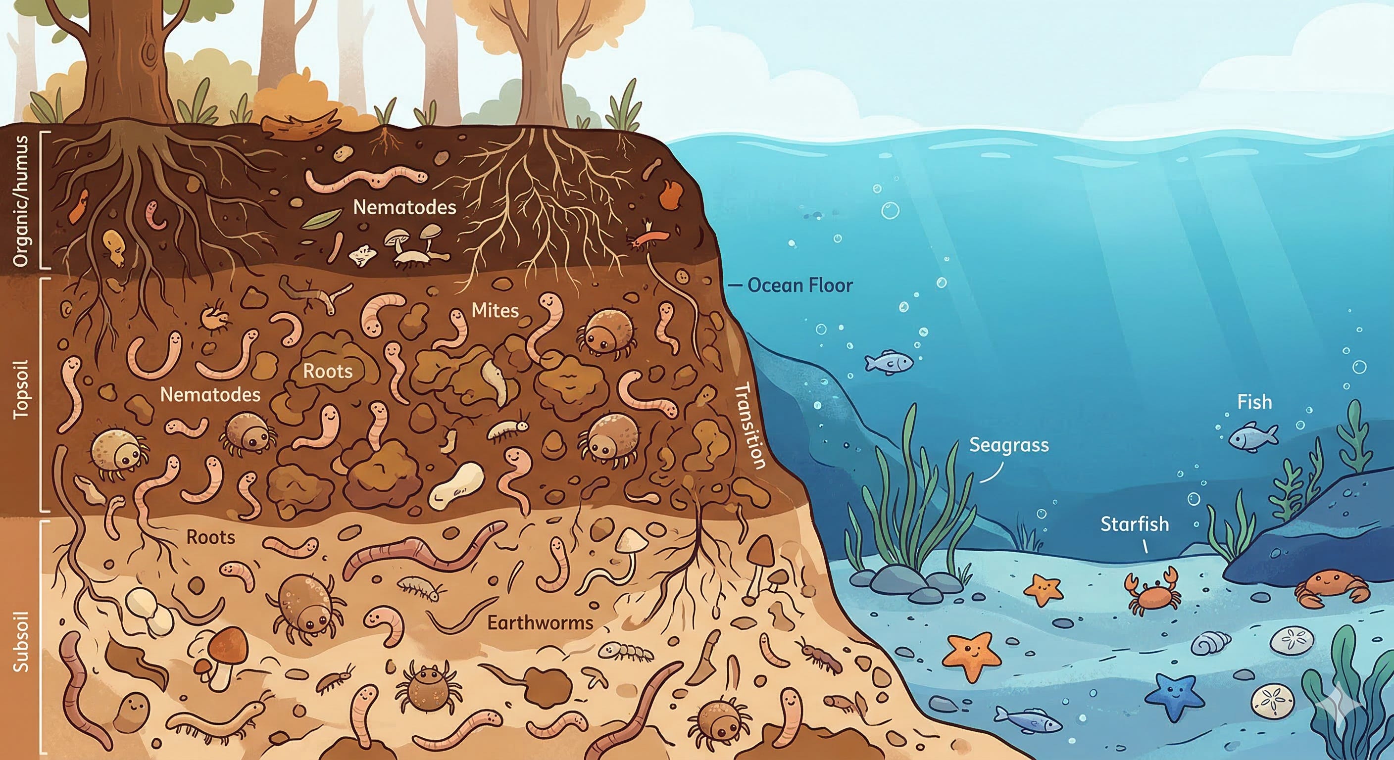
Terrestrial Soil Fauna
The foundational data comes from two landmark studies:
Van den Hoogen et al. (2019) estimated 4.4 × 10²⁰ nematodes in the top 15 cm of soil globally. Stefan Geisen, the second author, clarified that this accounts for roughly 90% of all soil nematodes, putting the total at about 4.89 × 10²⁰ (Grilo 2025a).
Rosenberg et al. (2023) estimated 10¹⁹ soil arthropods, of which roughly 95% are mites and springtails, with the remainder being ants, termites, and other groups.
For context: There are 8 billion humans and roughly 80 billion farmed land animals at any given time. Soil nematodes alone outnumber all farmed animals by a factor of 6 billion.
Marine Fauna
From Bar-On, Phillips, and Milo (2018):
Approximately 10²¹ marine nematodes – about 2× the number of soil nematodes.
Approximately 10²⁰ marine arthropods (copepods, krill, amphipods, etc.) – 10× the number of soil arthropods.
Marine nematodes are overwhelmingly benthic (living in seafloor sediment). Marine arthropods are split between benthic and pelagic (water column) habitats.
Density by Biome: The Terrestrial Landscape
Not all land is created equal. Rosenberg et al. (2023) provided mean densities of soil arthropods by biome. Grilo (2025a) combined these with van den Hoogen et al.’s nematode data to estimate total soil animal density. The results:
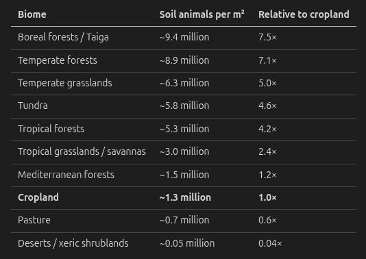
Several things jump out:
Forests are packed. Boreal and temperate forests have 7–8× the soil animal density of cropland. The mechanism is well understood: forests produce continuous, diverse leaf litter that feeds a complex soil food web. They have deep root networks supporting fungal communities that mites and springtails feed on. The soil is structured with pores and channels that provide habitat at every scale.
Cropland is relatively sparse. Tillage destroys soil structure. Monocultures reduce food web diversity. Pesticides directly kill a broad spectrum of fauna. The litter layer is minimal.
Pasture is sparser still. Grazing pressure, trampling, and simplified plant communities reduce below-ground complexity even further.
Deserts are comparatively empty. At 0.05 million per m², deserts have ~130× fewer soil animals than forests. Still even 50,000 animals per m² is impressive.
Volumetric Comparison: Soil vs. Sea
Since soil nematodes are measured in the top 15 cm (~0.15 m³ per m² of surface), we can convert to volumetric density and compare to marine environments.
One wrinkle: The dominant taxa change with the habitat. In soil, nematodes and arthropods (mites, springtails) coexist. In marine sediments, nematodes dominate overwhelmingly – they make up 80–90% of meiofauna (benthic organisms of 32–63 μm to 0.5–1 mm), with only small numbers of harpacticoid copepods alongside them. In the open water column, the situation reverses: There are essentially no pelagic nematodes (they are benthic animals, bound to sediment), and the invertebrate fauna is almost entirely arthropods – copepods, krill, and amphipods.
The table below uses “nematodes + arthropods” for all environments, but the composition varies as described:
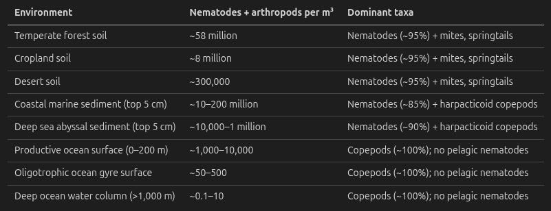
The key insight. Per cubic meter, terrestrial soil and some coastal marine sediments are by far the densest habitats per cubic meter for potentially suffering animals, though coastal sediment occupies a much thinner layer. The open ocean water column is orders of magnitude sparser – even productive surface waters have roughly 10,000× fewer organisms per m³ than forest soil. But the ocean’s total volume is vast (~1.37 × 10¹⁸ m³), so low per-m³ densities still add up to enormous total populations.
The deep ocean – both water column and sediment – is strikingly empty by terrestrial standards. It represents an enormous volume of near-zero-fauna space that already exists naturally.
What Drives Population Size? The NPP Primer
Understanding why some biomes have more soil fauna than others requires understanding net primary productivity (NPP).
NPP is the rate at which plants convert solar energy into organic matter, net of their own respiration. It’s measured in grams of carbon (gC) per m² per year. It’s an objective, species-independent measure of how much new biological material is being produced. A tropical rainforest has an NPP of ~1,000–2,000 gC/m²/yr. A desert has ~0–90 gC/m²/yr. Open ocean averages ~125 gC/m²/yr.
NPP matters because it determines the total energy flowing into the food web. More NPP means more food for decomposers, which means more food for the nematodes and mites that eat the decomposers, and so on up the trophic levels.
Vasco Grilo’s analysis found that NPP-related variables (biome type, soil organic matter) are far more important than any other factor in predicting soil fauna density. The m² -years of agricultural land per food-kg explained essentially 100% of the variance in welfare effects for his preferred parameters (Grilo 2025c).
A common misconception. NPP is not subjective to a species. When a cow eats grass, the NPP doesn’t change – the grass still produced the same amount of carbon. What changes is the pathway: instead of grass dying and feeding soil decomposers, the cow intercepts the energy, metabolizes 40–70% of it, and excretes the rest as dung. Dung is more labile (easier for bacteria to digest) than leaf litter, so it can boost local populations of bacterivorous nematodes around dung pats. But the cow has diverted most of the energy away from the soil food web, so the net effect on soil fauna is still strongly negative.
The same logic applies to any intervention that changes the pathway of NPP without changing NPP itself. This distinction turns out to be critical for evaluating pesticides.
An important caveat: Global NPP has barely changed. As I noted in part 1, Tomasik’s analysis of Krausmann et al. (2013) found that NPPeco – the global NPP available to wildlife – has barely changed over the 20th century, partly because CO₂ fertilization has increased potential NPP even as humans have appropriated more of it. This means that the biome-level density differences in the table above are real and actionable for local interventions, but the global total of animal metabolism may not have declined as much as defaunation indices suggest. Converting one hectare from forest to cropland genuinely reduces soil fauna on that hectare by ~7×; but globally, CO₂-driven NPP increases elsewhere may be partially offsetting these local reductions. This doesn’t undermine the case for targeted land use interventions – it just means we should be cautious about claims like “humanity has reduced total invertebrate suffering by X%.”
The Pesticide Trap
One might naively think that pesticides reduce invertebrate suffering by reducing their populations. But the relationship between pesticides and welfare is more complex – and possibly perverse.
Consider two interventions that both halve the standing population of soil fauna:
Intervention A: Reduce NPP by 50%. (For example, convert forest to desert, or shade the land.) The carrying capacity halves. At the new equilibrium, fewer organisms are born, fewer die, and the birth rate and death rate are both lower. Total deaths per year: lower.
Intervention B: Apply pesticides while keeping NPP the same. Food is still available. Organisms are born at rates close to the original (abundant resources encourage reproduction). But pesticides kill a large fraction of them. The population is suppressed below carrying capacity, but the high food availability keeps birth rates high. At the new equilibrium: birth rate is elevated (more food per capita), death rate is elevated (pesticides), and organisms are dying of pesticide poisoning instead of starvation or predation. Total deaths per year: much higher than the original, with deaths potentially involving more acute suffering.
This matters enormously for r-strategists. Brian Tomasik and Yew-Kwang Ng (1995) argued that for r-strategists, death is a large fraction of total lifetime suffering. If that’s right, the death rate may matter more than the standing population. And pesticides at constant NPP can increase the death rate – creating a high-throughput killing field rather than a genuinely smaller population.
Pesticide Persistence
The picture is further complicated by the fact that different pesticides have very different persistence profiles:
Organophosphates and carbamates degrade in days to weeks. These are closest to the “spray, kill, wash away, repeat” model – high-throughput killing.
Neonicotinoids persist in soil for months to years and are taken up systemically by plants. Any insect feeding on a treated plant gets a dose. This effectively makes NPP inaccessible to insects – the food is there but poisonous. This is closer to “reduced accessible NPP” and may genuinely reduce the carrying capacity.
Legacy organochlorines (DDT, dieldrin) persist for decades but are mostly banned.
The neonicotinoid case is the most interesting from a welfare perspective: by making plant material toxic, neonicotinoids functionally reduce the accessible NPP, which is closer to the “clean” intervention of actually reducing NPP. However, sublethal neonicotinoid exposure causes disorientation, impaired foraging, and reduced reproduction in insects – arguably adding suffering without the “benefit” of reducing the population.
Bottom line. Reducing actual NPP (through land use change) is a much cleaner intervention than applying pesticides at constant NPP. The famous ~75% decline in flying insect biomass in Germany (the Krefeld study) is attributed partly to pesticides and partly to habitat loss. From a welfare perspective, the habitat loss component (reduced accessible NPP) is straightforwardly population-reducing, while the pesticide component may be creating a high-throughput killing field.
A Better Metric: Life Expectancy at Birth
Let me flesh out the life expectancy at birth (LEB) metric for invertebrates, which I think deserves more attention. It’s a metric that we care about intuitively when thinking about humans, so it’s one that we have reason to also care about when it comes to other species.
LEB = total animal-years lived / total births per year
For an r-strategist marine fish laying 1 million eggs, of which 2 survive to reproduce, and average lifespan across all offspring is ~3 days: LEB ≈ 3 days.
For a K-strategist elephant with 6 offspring over a lifetime, of which 2 survive to reproduce, average lifespan ~20 years: LEB ≈ 20 years.
Why LEB is attractive.
It naturally penalizes the r-strategy horror: Systems where millions of beings are born just to die almost immediately get very low scores.
It’s legible. Most people intuitively understand that higher life expectancy is better.
It sidesteps the sign problem somewhat. You don’t need to know whether lives are net positive or negative to argue that ecosystems with higher LEB have less death per unit of ongoing life.
It aligns with antifrustrationism. Organisms born into very short lives full of pain score low, regardless of whether we think the brief pleasure before death was “worth it.”
Potential objections. A strict utilitarian would say this smuggles in the assumption that death is the primary locus of suffering. LEB doesn’t account for intensity of suffering during life. And it could be gamed by creating very long-lived organisms in terrible conditions. But as a rough heuristic for comparing wild ecosystems, it captures something real: Ecosystems dominated by K-strategists score higher than those dominated by r-strategists.
A refinement. One could weight by “fraction of lifespan spent with a developed nervous system” to exclude possibly non-sentient embryonic stages. For insects that undergo complete metamorphosis, eggs are probably not sentient, but larvae have functional nervous systems from early instars. For nematodes, the L1 larva hatches with 222 of its final 302 neurons and is immediately mobile and responsive – so the cutoff would be at hatching. The European Food Safety Authority (EFSA) suggests the onset of potential sentience at roughly “the beginning of the last third of development within the egg or mother” for most vertebrates, and “when it is capable of feeding independently” for fish, amphibians, and invertebrates (EFSA 2005).
The Ocean: Acidification as Accidental Intervention
One of the largest ongoing shifts in marine invertebrate populations is driven by ocean acidification – an accidental consequence of CO₂ emissions.
The mechanism. CO₂ dissolves in seawater and forms carbonic acid, lowering pH. This reduces the availability of carbonate ions that many marine arthropods need to build shells and exoskeletons. Calcifying species – copepods, pteropods, krill, crabs – are directly harmed. The effect is already measurable: ocean pH has dropped by about 0.1 units since the Industrial Revolution and is projected to drop another 0.3–0.4 units by 2100 under high-emission scenarios.
Does acidification reduce total populations, or just reshuffle species? At the current margin, acidification appears to be reducing total marine arthropod populations rather than merely substituting non-calcifying species for calcifying ones. The reasons:
Timescale mismatch. Current acidification is happening over decades; evolutionary adaptation takes millennia to millions of years. Non-calcifying species haven’t had time to evolve into vacated niches.
Structural role of calcifiers. Copepods and pteropods occupy dominant roles in marine food webs. Their decline disrupts the entire ecosystem, not just their specific niche.
Paleoceanographic evidence. After the Paleocene-Eocene Thermal Maximum (PETM, ~56 million years ago), which involved rapid ocean acidification, it took ~100,000–200,000 years for marine communities to reorganize. Recovery was slow and involved reduced overall productivity.
This makes ocean acidification one of the few large-scale ongoing processes that is plausibly reducing total marine invertebrate populations.
Dead Zones: More Nutrients, Less Life
Another counterintuitive marine phenomenon: nutrient runoff from agriculture creates “dead zones” that dramatically reduce animal life.
The mechanism. Nitrogen and phosphorus from fertilizer enter coastal waters → algal bloom at the surface → algae die and sink → bacterial decomposition of sinking algae consumes enormous amounts of dissolved oxygen → oxygen drops below ~2 mg/L (well-oxygenated water has ~8 mg/L) → most animals suffocate.
The Gulf of Mexico dead zone, fed by Mississippi River agricultural runoff, covers ~15,000 km² of seafloor with severely depleted macrofauna every summer.
Dead zones vs. pesticides. An established dead zone is more like “reduced NPP” than like “pesticides at constant NPP”: Within the anoxic zone, the carrying capacity for macrofauna is near zero, so there’s no high-throughput killing. The suffering is concentrated in the creation and seasonal re-establishment of the dead zone. Permanent dead zones (rare but possible) would be functionally equivalent to removing the habitat – genuinely low birth rate and low death rate, not a killing field.
However, many dead zones are seasonal – forming in summer and dissipating in winter. This seasonal cycling creates recurring mass mortality events, which is the oscillating-biome problem: not a stable low-population state, but a perpetual cycle of colonization and die-off.
Grilo’s Key Findings
Vasco Grilo’s analyses are dense with inline math, which can make the key insights hard to extract. Here’s a plain-language summary of what I consider his most important findings:
1. Effects on soil animals might dwarf effects on intended beneficiaries. Grilo’s earlier models indicated that the impact on soil nematodes, mites, and springtails is orders of magnitude larger than the impact on the people or farmed animals the intervention is designed to help. He has since updated these models, and commented on my previous article that his new credible intervals span many orders of magnitude in both directions, extreme uncertainty that is driven by uncertainty over nematodes’ welfare ranges.
For [some reasonable parameters], I estimate that GiveWell’s top charities change the welfare of soil ants, termites, springtails, mites, and nematodes [10⁻⁵ to 10¹⁰] times as much as they increase the welfare of humans. For my preferred [parameters], the change in the welfare on those soil invertebrates is 41.5 times … the increase in the welfare of humans ….
Note that if the GiveWell numbers are based on increases in human population, then they are questionable due to both Krausmann et al. (see above) and Roodman (2014).
2. Agricultural land has fewer soil animals. Crops have ~1.3 million soil animals per m², compared to ~3–9 million for natural biomes. Pasture has even fewer (~0.7 million). So anything that increases agricultural land – including saving human lives, which increases food demand and therefore cropland – reduces, at first approximation, soil animal populations.
Grilo clarifies in a comment that this is only true of arthropods:
I think agricultural land has less soil arthropods, but I have little idea about whether it has more or less soil nematodes. The vast majority of soil animals are nematodes. So I also have little idea about whether agricultural land has more or less soil animals.
3. Nematodes dominate. Of the total welfare effect on soil animals, 90–94% comes from changes in nematode populations, depending on the biome. This is because nematodes outnumber arthropods ~50:1. It depends mostly on the welfare ranges whether this numerical advantage overwhelms everything else.
4. The sign is uncertain. Grilo estimates nematodes have negative lives with probability ~59%, mites ~56%, springtails ~55%. If their lives are net negative, reducing their populations (via increasing agricultural land) is beneficial. If net positive, it’s harmful. Every concrete recommendation flips depending on this sign. Grilo’s own best guess is net negative, but he explicitly acknowledges the uncertainty.
5. Land use is the key variable. The m²-years of agricultural land per food-kg explain essentially all of the variance in welfare effects across different foods and interventions. Beef requires ~326 m²-year/food-kg; chicken requires ~12; peas require ~7.5; soy milk requires ~0.7. From the soil-animal perspective, producing 1 kg of beef reduces soil-animal-years by ~1.39 billion – 164 billion times as much as it increases the living time of the cows.
These findings are robust to a wide range of assumptions about welfare ranges, as Grilo demonstrates with sensitivity analyses across different exponents for the neuron-count-to-welfare-range relationship (Grilo 2025c).
Summary
The empirical landscape boils down to a few key facts:
Soil fauna are staggeringly abundant – 10²⁰ nematodes, 10¹⁹ arthropods – and their total expected welfare dominates that of all other animal groups combined if they are sentient.
Population density varies enormously by biome, from ~9 million per m² in boreal forests to ~50,000 per m² in deserts. Land use change is a powerful lever. But note that the oft-cited difference between croplands and forests is only around 1–8×.
Reducing NPP is a cleaner intervention than pesticides for lowering populations. Pesticides at constant NPP risk creating a high-throughput killing field rather than a genuinely smaller population.
Life expectancy at birth may be a more informative metric than total animal-years, especially for r-strategists where death is the dominant source of suffering.
Ocean acidification and dead zones are reducing marine invertebrate populations, but the mechanisms and welfare implications are complex.
Land use explains almost everything in Grilo’s analysis. If you want to affect soil fauna populations – in either direction – the most powerful lever is changing how land is used.
In part 3, I’ll turn to the practical question: Given all of this, what should we actually do?

Hi Dawn. Thanks for looking into soil invertebrates, and my posts.
"One might naively think that pesticides reduce invertebrate suffering by reducing their populations. But the relationship between pesticides and welfare is more complex – and possibly perverse."
I do not think pesticides would robustly decrease suffering even if they only changed the population of soil invertebrates, and not their welfare per animal-year (https://forum.effectivealtruism.org/posts/pEbiEmeu2agEHJgyu/a-database-of-near-term-interventions-for-wild-animals?commentId=r7bCtdh8MWp2J9jqi).
"1. Effects on soil animals dwarf effects on intended beneficiaries."
I can see this being the case, but I am also open to effects on soil animals being negligible (https://forum.effectivealtruism.org/posts/L9NZGB7xbxiwgndPk/welfare-biology-and-ai-the-quiz?commentId=wMx8KvXzPBdGMvc9M).
"2. Agricultural land has fewer soil animals."
I think agricultural land has less soil arthropods, but I have little idea about whether it has more or less soil nematodes (https://forum.effectivealtruism.org/posts/WbmDhpqKcT8gjwpso/saving-human-lives-cheaply-is-the-most-cost-effective-way-of?commentId=yx6pS5mbjksiGp8fg). The vast majority of soil animals are nematodes. So I also have little idea about whether agricultural land has more or less soil animals.
"3. Nematodes dominate."
This is my best guess, but it is very uncertain. I would not be surprised if effects on soil nematodes were negligible compared with effects on soil arthropods.